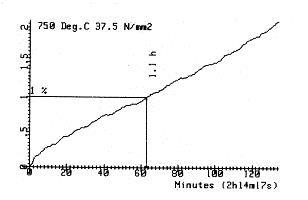
INTRODUCTION

While Big History has only been named as such within the last few decades, [1-3] its recent analysts have recognized their indebtedness to Alexander von Humboldt, H. G. Wells and others from earlier generations. [4,5] I remember having day-dreamed when I was 14 that it would be nice to be able to narrate the evolution of my family over say 30 or 50 generations to understand my immediate, present day family. I found appealing the idea that there would be connections between the past and more recent events in this family. My goal was to see how earlier generations continued to exert their influence. I would search for a long path from what this family started with and went through to what this family had become after centuries. This was my « big history » dream!

Later, I earned an engineering degree after having studied several scientific subjects in a rather compartmentalized way. These studies allowed me to go deeply into well defined and focused scientific fields. I gained an understanding of the state-of-art methods and how science proceeds slowly, step by step.

I have more recently sought to integrate the musings of my youth with how different fields can be put together in a global approach of aging and evolution to produce a « big history » perspective. 

1.     FROM CREEP TO THE RELIABILITY OF SYSTEMS

After my education, I worked in a research centre studying creep of steels at very high temperatures (1473 – 1523 K); I focused on this field even though the topic usually receives brief attention in most curricula.. Creep is the slow deformation of materials under stress at given temperature. It is usually taught very briefly in the field of physical metallurgy; it is often given about ½ hour in a 5 years engineering programme.

Afterwards, I went into a licensed inspection agency and was involved in the follow-up of fossil-fired thermal power plants. In those times, the issue at stake was the residual life assessment of that kind of plant. These plants had been designed for their thermal components (boiler, pipes, headers, turbine …) to operate during 100,000 hours under creep at around 813 K (or more). However, as they reached this time limit seemingly in good working order, it was not clear if they could be operated any longer. How could their residual life beyond 100,000 hours be assessed? So I started investigating creep curves for temperatures of the order 813 K and was astonished to find that although the microscopic structure of the metal was completely different in function of the temperature, the creep curves were alike for 813 K and 1473 K. For instance, the crystalline microstructure is face-centered cubic at 1473 K and body-centered cubic at 813 K, the mechanism of creep was different, the diffusion of atoms and vacancies in the microstructure varied a lot, etc. But the creep curves were alike in shape. Only the duration of the process was strongly different : of the order of 100,000 hours at 813 K and of a few seconds at 1473 K. Figure 1 shows a typical creep curve.

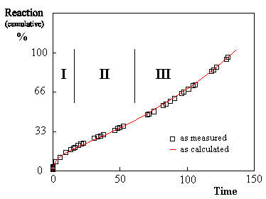
Figure 1 Creep curve of a steel at higher temperature showing three stages : I) a first concave part (« primary creep ») followed by II) a quasi-linear part (« secondary creep ») and III) a third convex part (« tertiary creep »), before rupture (arbitrary units).

This kind of curve is found in the creep of metals subjected to load or stress [1] at higher temperature (only the first part is seen at lower temperature). It can be interpreted as follows : (1) firstly, after the « shock » of being put under stress by the testing machine, the test piece shows a progressive adaptation : it is strained and the strain curve (the curve reflecting the « reaction » in Figure 1) is concave from below (« primary creep »). This stage is followed by (2) a second stage called « steady or stationary stage », where there is a balance between the defence reaction (strain) and the defects caused by the stress; the strain curve is (quasi-)linear. If the stress is maintained, (3) a final stage develops with the exhaustion of the test piece up to rupture ; the strain curve is then convex from below. 

In course of further investigations, it appeared that a good mathematical description of such creep curves was given by following equation for the strain [7-10]:

    (1)

With :

k > 0
0 < α << β < 1
t : time (s)
k can be related to the applied stress « σ » by the expression:
k’, b, α and β are constants at given temperature, metallic structure and composition (they may change when temperature and/or metallic structure and composition change).

Because of the multidisciplinary approach adopted in the present article, I’ll make use of the diphthong letter Æ(t) to express that it is a measured parameter reflecting an « Aging » or an « Evolution » which develops in function of time (the reason for this choice of words will become obvious in the course of the text). In the case of creep, this measured parameter Æ(t) is the creep strain.

Equation (1) is not the more frequent manner of describing creep curves. The usual way consists in focusing on the stages themselves, e.g.: for the first concave part of the curve [11], for the second linear part of the curve corresponding to the secondary creep [12], which is called the « useful life » in practical applications, and a growing exponential for the tertiary creep, etc.

But Equation (1) has the advantage to combine all three stages. Moreover, in addition to fitting creep curves, it allows to easily derive a formula for the classical vs. (logarithm of the stress vs. logarithm of the rupture time) diagrams [13,14] as widely used in design standards, what the default presentation can not. And as we shall see, Equation (1) will also allow for comparisons with observations in other fields.

Indeed the derivative of Equation (1) gives the strain rate in function of time :

   (2)

The shape of the corresponding curve is shown on Figure 2. The first part of the curve (for small times, i.e. when ) is like the learning curve of Duane [15].

Several observations were made by Duane in the 1960’s. He investigated repairable mechanical systems and found that their failure rate () always obeyed a law of decrease with time:

This meant that the number of failures of the system over a period of time decreased when time was going on. This behavior induced the feeling that the system had ”learned” from its past experience and had found solutions to make less mistakes. Therefore, Duane called this behavior ”learning” and the curve given by : the ”learning curve”. He found that, in general, one had:

The systems considered were repairable mechanical devices such as airplane generators, submarine diesel engines, hydromechanical appliances.

Other authors after Duane reported similar behavior on a broad range of devices, e.g. loading cranes [16], army trucks [17] etc. and it is since then a widely accepted evidence that the learning curve can be observed on many operating mechanical devices, but also electr(on)ical devices, etc.

Using Equation (1), Equation (2) can also be written:

   (2')

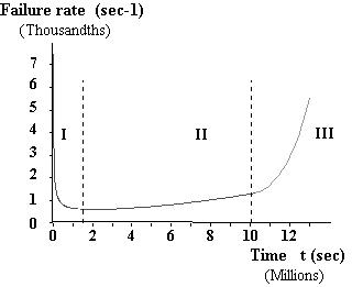
It is noteworthy that Figure 2 is the derivative of the creep curve but also shows a typical « bathtub curve » as known in the reliability analysis of mechanical, electrical, … systems. This kind of curves is found for a lot of systems : engines, cars, …. During the life of these systems, there is a first phase of adaptation where the failure rate is first elevated and decreases (« infant illnesses »). Then the failure rate is around a minimum (« true life »). After a time, the failure rate starts to increase again first slowly then more steeply up to collapse of the system (« aging »).

Figure 2 Typical bathtub curve (arbitrary units)

In the frame of reliability analyses of systems, Equation (2) can be seen as the failure rate for a modified Weibull distribution [18,19]. The modification lies in the adding of an factor. The Weibull distribution is found back when α is put = 0. This modified Weibull distribution may be considered as a generalization of many other models [20]. Observe that the failure rate function of Equation (2) can be considered as a sum of two Lee’s failure rate functions [21] by noting :

    (3)

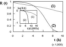
where k^*:= α.k/(β + 1), β^*:= β + 1 [21]. The parameter β is called the characteristic of the system. When α = 0, the model reduces to a Weibull process ; when α = 0 and β = 2, the model reduces to the Rayleigh process ; when β = 1 and α.t is very small, the model is approximately an exponential model. When β = 0, the model reduces to a type I extreme-value model, also known as a log-gamma model. As pointed out in [22], the model can be considered as a limiting process of the Beta integrated model introduced in [23].

The reliability corresponding to the bathtub curve model given by Equation (2) is by definition given by Equation (4) and visualized on Figure 3[2].

   (4)

Figure 3 - Examples of reliability curves.
The system is fully reliable in the beginning (, but with the time going its reliability decreases, first slowly then steeply down to zero.

The loads/stressors in mechanical and electr(on)ical devices are the constraints and environmental challenges due to operating.

2.     GROWTH AND DECLINE CURVES

In the same way that allows the reliability to be given by the exponential of minus the « creep curve », interesting curves are obtained using the exponential of minus the « bathtub curve ». We shall call such curves « growth and decline curves » (GD-curves)[3]. Following equation is used :

(5)

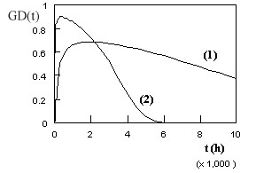
Where : « c » or « C’ » are constants > 0 and can be = 1 ([4])

Growth and decline curves (GD-curves) are found in constant strain rate tensile tests (CSRTT) of metals at high temperature. These tests are the counterpart of creep tests. During creep, the stress/load is constant and the strain is recorded. Then the strain rate varies as shown by the bathtub curve. In CSRTT, the strain rate is maintained constant and the load is recorded. This gives GD-curves. As seen on Figure 4, these curves show three stages : (1) first there is an increase of a « capacity », then (2) the curve reaches a maximum (peak) before to (3) progressively decline to levels encountered in the first stage. This is like climbing and descending an hill. Two typical shapes are given on Figure 4. However, the shape can be different - with e.g. smoother growth and steeper decline - in function of the values of the constants « c » and « C’ ».

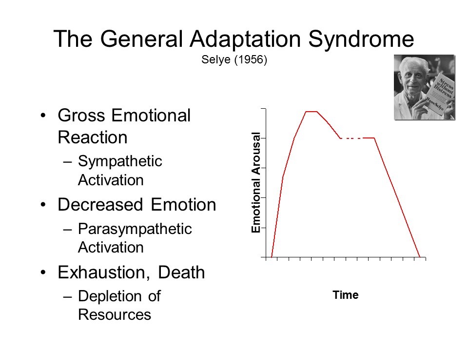
Figure 4 - Examples of growth and decline curves.

As will be seen later on in the text, GD-curves are also found in biology and astronomy, and probably in other fields.

3.     FROM RELIABILITY TO BIOLOGY

When one reads the descriptions by Hans Selye [24-28] and others of the General Adaptation Syndrome (G.A.S.) they are - mutatis mutandi - astonishingly close to the way creep curves would be described.

The G.A.S. is the non specific reaction of the biological system to external attack. Let us give the word to Hans Selye :”...[the general adaptation] syndrome is...[an]...expression of general defence divided into three stages. During the first, or acute stage,observed in the rat ordinarily 6 to 48 hours after the initial injury, one notes a rapid decrease in the size of the thymus, spleen, lymph glands and liver...After a few days, however, a certain resistance is built up against the damaging stimulus...the animals became resistant...If ...[the stressors]...were continued still longer the animals lost their resistance, and in a third stage died with organ changes similar to those seen in the first stage...We have termed...[the] 3 stages: the stage of alarm, the stage of resistance and the stage of exhaustion...”[25] (emphasis added).

Concerning the human body, one can refer to the summary given by the Counselling Connexion (the Official Blog of the Australian Institute of Professional Counsellors) [29]. It starts with the words :

“The G.A.S. describes a three stage reaction to stress: (1) initial alarm / reaction to the stressor, (2) resistance / adaptation to coping and (3) eventual exhaustion.”

In addition, it is noteworthy that Selye made a correlation between the G.A.S. and aging [27].

Reading such kind of descriptions and features pushed me decide to earn an additional degree in molecular biology.

A way to visualize the G.A.S. is shown on Figure 5.

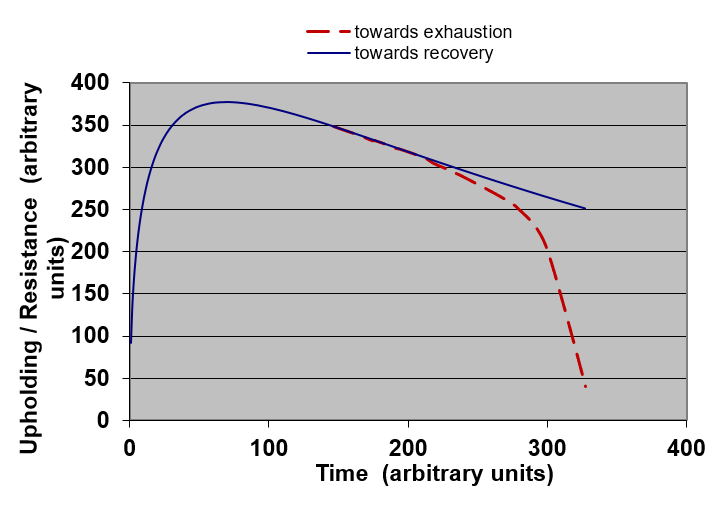
Figure 5. Example of representation of the General Adaptation Syndrome (found on Internet).

This is similar to a growth and decline curve. Probably with precise measurements, one would get a curve like the one shown in Figure 6.

Figure 6. Example of representation of the General Adaptation Syndrome following Equation (5) – The blue plain curve corresponds with Equation (5) when the stressor holds but is sufficiently low to allow the system to recover after removal of the stressor – The red interrupted curve shows what happens when the stressor is that high that the system will soon be harmed and subject to premature exhaustion.

This induced to think that there would probably also exist curves of the kind bathtub curve, reliability curve or creep-like curve to be found in biology as far as aging and evolution are concerned. And indeed a lot of examples are found in the literature.

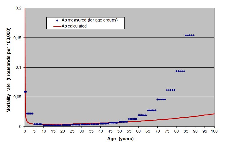
Just to start with mentioning all curves currently called « mortality curves » which are in fact bathtub curves, see e.g. Figure 7. Mortality curves give the rate of mortality of a population in function of the age. They thus also reflect the probability of death at a given age of a lambda individual in this population. This is equivalent to the failure rate of systems as given by the bathtub curve. The fact that the increase of mortality rate is quicker as measured than as calculated is an often seen feature. As will be noticed later on, it is due to the fact that instability can settle after a time  (instability time) from which the growing exponential in Equation (1) and (2) becomes higher than « e »[5].

Figure 7. Mortality rates per 100,000 for women in China by age group for the year 1957 [30]. Rhombs correspond to recordings per age group. The plain line is obtained using Equation (2).

And all « survival curves » or « survivorship curves » found in biology are in fact reliability curves, see e.g. Figure 8.

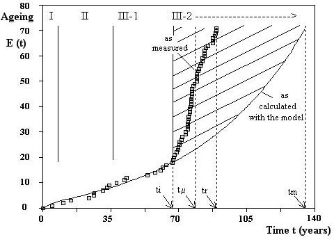
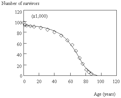
Figure 8. Survival curve of United States whites for the period 1929-1931 [31]. The rhombs correspond to empirical data while the plain line is obtained using Equation (4).

But creep-like curves are also found, e.g. in tumour growth as shown on Figure 9.

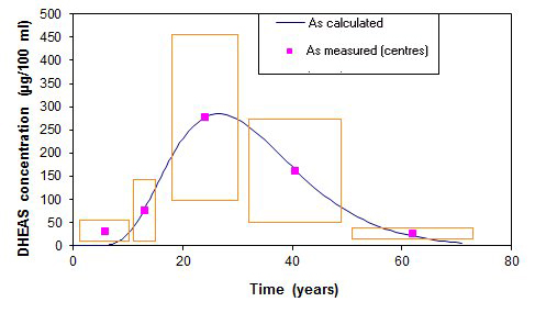
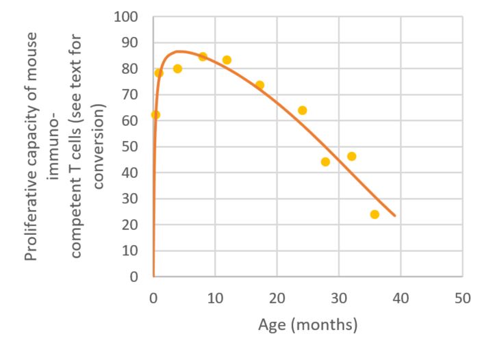
Figure 9. Growth of Meth-A sarcoma tumours induced in mice [32]. Squares correspond to measured values. The plain line is obtained using Equation (1) (time in seconds).

And finally, growth and decline curves are encountered in biology as already shown by the example of the G.A.S., but also in several other cases : changes in bone mass [33], muscular force [34], maximal oxygen uptake in healthy fit men [35], incidental memory scores [36], cumulative increase in human diploid fibroblast cells number [37], immune functions (e.g. antibody formation) in humans and animals, …Each time there is (1) an increase of a « capacity » (the bone mass, the muscular force, the maximal oxygen uptake, incidental memory scores, immune functions, average speed of sprinter on 100 meters, etc. etc.) up to a maximum where (2) it is about maintained a while in a steady-state. Then (3) the « capacity » starts to diminish first slowly then more and more quickly with the time going.  

Two further examples are given below :

1) From the pioneer work of Baulieu [38], the dehydroepiandrosterone sulfate (DHEAS, a kidney produced hormone) concentration in human serum has been considered a good marker for the aging of humans [39] [40]. Figure 10 gives the DHEAS levels of normal males and females plotted against age [40]. Measurements have been made on 25 children, 32 adult males and 42 adult females. In order to get a better view, only the centres of the rectangles corresponding to the zones of measured values are shown, together with the rectangles. One observes that, after a first increase, the DHEAS content in plasma reaches a peak around an age of twenty five then continuously decreases. The plain line corresponds to the computations using Equation (5) and c=1.

2) The decline in phytohemagglutinin responsiveness of spleen cells from aged mice was measured by Hori et al. via recording the in vitro proliferative capacity of immunocompetent T-cells (by [³H]Tdr incorporation in Δ cpm) [41]. The results are summarized in Figure 11. Dots correspond to experimental averages as taken from [41]. The plain curve was obtained by fitting the data with Equation (5) and c=1. The values in ordinate can be converted into Δ cpm by using the conversion: .

In summary, Æ(t) in biology describes the cumulative aging of a given system, the mortality curve , the survival curve and the growth and decline curve (of a capacity, a resistance, …).­

The loads/stressors in biological systems are the constraints and environmental challenges due to living. For instance, sub-citotoxic stresses can be experimentally imposed on cells in vitro to get accelerated aging curves (the « stress » would then be in parameter « k » of Equation (1) and the influence of the imposed « stress » on the value of « k » can be inferred).

Figure 10. Dehydroepiandrosterone sulfate (DHEAS) concentration in human serum in function of age.

Figure 11. In vitro proliferation of mouse immunocompetent T-cells in function of age.

4.   FROM CREEP TO (NEO-)DARWINIAN EVOLUTION

We check Equation (1) to (3) in the framework of (Neo-)Darwinian evolution. 

One should not be astonished that it is spoken of reliability in the context of (neo-)Darwinian evolution, as it is exactly what nature is driving at : that the fittest species for a given environment will thrive, thus will prove a sufficient level of reliability. Evolution is prone to preserve the integrity of the better adapted species (e. g. for eukaryotes : stable DNA to be read many times but protected into a nucleus, double membrane of cells, …). The living entity has an organization that reveals selective advantage in its life environment. There it is armed to reliably survive. Moreover, some reliability is always needed in connection with making evolutionary attempts successful : entities and species would otherwise disapp­ear all too quickly.

Let us now check whether curves of the kind shown in Figure 1 can be found in connection with evolutionary data. This would suggest that evolution and aging are two faces of the same coin.

In 1975, Nei obtained a rough relationship between the number of nucleotide pairs (bp) in the DNA of different species and their reckoned time of appearance on Earth [42]:

       (6)

with α := 2.3 10^-9years^-1 for an estimated 3 10⁹ years elapsed from bacterium to mammal (n₀ is the initial DNA content, taken here as having the value n₀ := 4 10⁶bp which corresponds to E.coli). Equation (6) is equivalent to Equation (1) where β is put β = 0.

Equation (6) can be re-written in natural logarithms :

                                (7)

The same can be done for Equation (1) :

        (8)

Assuming life to exist on Earth since about 3.5 10⁹years (taken as time zero) and considering the time of appearance of living entities as shown in Table 1, one may compare the results using Equation (7) (with α := 2.3 10^-9years^-1and n₀ := 4 10⁶ bp), and Equation (1) (with α := 2.3 10^-9years^-1 , β := 0.45 and k = 5.755).

Both Equation (7) and Equation (8) fit the points as can be seen on Figure 12 (ordinate in natural logarithm scale).

Table 1 – Time of appearance of living entities on Earth and their number of nucleotide pairs (bp) [42]

Case	Type of living entity	n0 (bp)	After (years) :
(1)	E.coli	4 106	2 108
(2)	First unicellulars (e.g. Neurospora)	4 107	1.2 109
(3)	Bony fish	9 108	2.6 109
(4)	First mammals	3.2 109	3.1 109

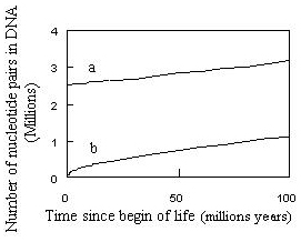
However, as can be seen from the start of the curves using Equation (1) and Equation (7) (see Figure 13 where the ordinate is no longer in natural logarithm scale), extrapolating back to time zero gives a predicted value of more than 2 10⁶bp (exactly 2 525 134 bp) using Nei’s equation. That such a big number of nucleotide pairs would already exist in the genome of all living entities in the very first forms of life on Earth seems unrealistic. On the contrary, using Equation (1) allows to start from small molecules as has most probably been the case (the computation gives 0 bp at time t :=0 ; 229 bp after 1 year ; etc.)

Whatever the model, the curve should start from a value close to or equal to zero.

Figure 12. Number of nucleotide pairs (bp) in genome as a function of time from the start of life on Earth : (a) As calculated using Nei’s equation – here Equation (7) ; (b) As calculated using Equation (8). Squares correspond to 4 species as selected by Nei [42].

Figure 13. Start of the curves of Figure 12 (but with the ordinate no longer in logarithmic scale): (a) As calculated using Nei’s equation – here Equation (6) - (b) As calculated using Equation (1).

Using Equation (1), one better understands why the increase was so quick in the first million years (as noticed by e.g. de Duve [43]) and slowed down afterwards : an initial quick evolution followed by a decrease of the evolution rate is a typical shape for the first stage of evolution curves as given by Equation (1).

Now, the question rises : if the evolution curve is given by Equation (1), has it to be smooth ?

Phyletic gradualism goes in the direction of a systematic gradual evolution. This does not necessarily mean that the evolution curve must therefore be smooth at all scales. In reality, in the cases where Equation (1) applies, the curves should only be smooth at higher time scales as compared to the default duration of the process. When one concentrates on smaller periods of the process, smoothness would disappear. Irregular alternate periods of increase, stabilizing and sometimes even decrease would be seen. This is because adaptation to « stress » implies that there is a time component. Electro-chemical transfers of information, chemical reactions, cell divisions, DNA transcriptions, reactions to unexpected shocks, reactions after learning, …., all these adaptive and genetic actions or reactions need time even if very short: they cannot take place instantaneously. Adaptive efforts appear within the system to allow its further working. This is time (and energy) consuming. There are attempts, initial responses may miscarry or reveal inadequate, there are delays, stabilization is sometimes needed, coordination is not always perfect, … As the system is open, it can have problems of provisioning, getting energy sources, needed stuff is not (immediately) available, stressing agents may suddenly concentrate, … This all makes that the evolution curve shows signs of « hiccup ».

Figure 14. First part of a creep curve (with permission of Laborelec).

Even in the case of the creep curve of metals (see chapter 1 above), the curve of Figure 1, is not perfectly smooth when one observes it in details. An example is given in Figure 14. Actually there are little steps, small periods of stabilization (stagnancy), asymmetries, … 

Also concerning the evolution of species, favourable solutions take time to spread to a whole population. Even when occurring quickly (e.g. resistance of bacteria to antibiotics), a finite time is needed.

In summary, one expects the process of evolution not to develop very smoothly but rather ”step by step” even if at large scales it could be seen as continuous in first approximation. This is schematized in Figure 15.

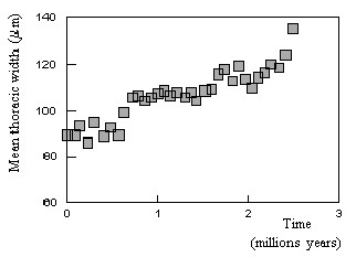
Figure 15. Examples of « step by step » evolutions (schematic). Curve ”a” corresponds to an evolution at a rather regular pace. Curves ”b” and ”c” describe evolutions which are slow in the beginning and show periods of stagnancy (longer for ”c” than for ”b”) without apparent evolution. Curve ”d” is typical for a quick evolution in the beginning which results in a shorter duration of the process.

As shown in Figure 16, the actual evolution curve which is observed on Earth for the period starting 600 millions years ago[6], is rather a curve of the types « b » or « c » in Figure 15. In spite of five mass extinctions and several more reduced extinctions, the curve of Figure 16 giving the number of taxonomic families (taken as marker for the evolution of species) in function of time shows an evolution in three stages similar to the curve of Figure 1. The periods of extinction resulted in « stagnancy » as not the totality of species were extinct then and new species appeared.

The idea of « step by step » evolution as reflected by « hiccups » in the evolution curve is in line with « punctuated equilibrium » [45]. The adaptations are not instantaneous. Evolution works by fits and starts at small scale. There are periods of changes and periods of consolidation, spreading of the gained selective advantages in the population and thriving. Therefore at the right scale, step-like curves would be observed.  

Figure 17 gives an example of punctuated equilibrium as re-drawn from [46] and quoted by [45]. It shows the evolution of the mean thoracic width of the antarctic radiolarian Pseudocubus vema over 2.5 millions of years from the advent of the first samples. Similarly to the curves of Figure 15 and Figure 16 one observes periods of stagnancy between the periods of increase.

Figure 16 Extinction rate (blue curve) and evolution of the number of families (red curve) over the last 600 millions of years [44].

Finally, it is interesting to draw a parallel with the experimental work of Lenski [47] and Elena [48]. These teams recorded evolutionary changes in bacterial populations (E. coli) propagated for 10 000 generations in identical environments. They first found that the cell volume and the relative fitness (to the ancestor) grew according to a concave (from below) curve [47]. Such curves are similar to the beginning of the curve in Figure 1. But, focusing on a population at a smaller time scale (3 000 generations), they got a better fit with a step-like model, what they considered to show evidence of punctuated equilibrium [48]. This work has since been continued up to 50 000 generations which is an inestimable source of information on in vitro evolution [49][50].

More details on the biological issues related to aging and evolution can be found in [51], [52] and [6].

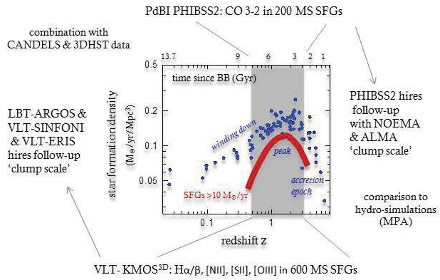
Figure 17. Example of punctuated equilibrium. Evolution of the mean thoracic width of the antarctic radiolarian Pseudocubus vema over 2.5 millions of years from the advent of the first samples (re-drawn from [46] as quoted by Eldredge and Gould [45]).

5.  APPLICATIONS IN ASTRONOMY AND THE EVOLUTION OF THE UNIVERSE

Stars and galaxies have a life. The life of stars can also be divided into 3 stages (with sub-stages): (1) a stage of formation of the star ; (2) a stationary stage of true life (where the fuel in the star is used to maintain its life); (3) a final stage after the whole fuel has been burnt, where the star’s life goes to end : black hole, neutron star, supernova or white dwarf in function of its mass. The aging of stars is usually analysed with the Hertzsprung – Russell diagram. However it is not possible to extract data from this diagram to find the parameters as described in the present article.

Concerning galaxies, I have found very few information which could become integrated in the present point of view, but it is interesting to notice that galaxies also have a life with infancy, maturity and senescence. For instance, Figure 18 taken from [53] shows the star formation density of « main sequence » star forming galaxies (10 solar masses / yr) in function of time since the Big Bang (BB)[7] : see upper abscissa. Here the evolution is to be read from right (Big Bang) to left, corresponding to now (13.7 Gyrs after the BB). The blue points correspond to the observations. They form a global curve which shows the shape of a GD-curve as put into evidence by the schematic thick red line. In fact, reading the cloud of blue points from right to left, i.e. from the BB to present time, we see that it nicely follows a curve of the kind shown for a GD-curve in Figure 4, 6 or 11 above. In this case, the « capacity » would be that of forming stars. The peak would be around 3 - 6 Gyrs. However, this interpretation is still speculative as the issue should first be investigated on base of the existing models and computations for the formation and evolution of galaxies.

Figure 18. Star formation density of « main sequence » star forming galaxies in function of time since the Big Bang (BB): to be read from right (BB) to left (now). Taken from [53] page 16.

Now concerning the evolution of the Universe, let us first cite the cosmologist who has been at the roots of the BB idea, G. Lemaître : ”...If the world has begun with a single quantum, the notions of space and time would altogether fail to have any meaning at the beginning ... Clearly the initial quantum could not conceal in itself the whole course of evolution ... The whole matter of the world must have been present at the beginning, but the story it has to tell may be written step by step.”(these words are taken from a seminal text published by G. Lemaître in 1931 in Nature [54]).

As is well known, the classical approach of the evolution of the Universe is based on Einstein’s field equations [55] as usually reduced using Robertson–Walker metrics and on the available measurements (I_asupernovae redshifts, cosmic microwave background radiation – CMBR, satellite missions – Cobe …). It follows an hot BB flat Universe scenario. Using Friedmann-Lemaître-Robertson-Walker (FLRW) models, it is thought that the Universe started from an hot BB and expanded into a radiation-dominated era up to the emission of the CMBR (around 380,000 years after the BB), followed by a matter-dominated era of about 13.4 billions years up to present time. A stage of inflation (around 10^-35 to 10^-32 s after the BB) is also assumed as it explains empirical data which are otherwise difficult to explain like the homogeneity and the flatness of the Universe. The cosmological constant Λ, initially introduced by Einstein in his equations to allow a non-evolving Universe was firstly put =0 in front of the evidence of the expansion.

In connection with the present text, it is interesting to focus on the Hubble parameter « H » which gives the recession velocity of galaxies divided by their distance. This is usually expressed using the distance scale factor « R » by:

;                                            (9)

Computations give then :  (for the inflationary stage),  (for the radiation-dominated era) and  (for the matter-dominated era)[8].

This could be summarized in following equation:

                    (10)

With during the radiation-dominated era and during the matter-dominated era.

This makes sense as integrating Equation (10) results in a distance scale factor  giving (typical for an inflationary stage) for and  (with  typical for the radiation- and matter-dominated stages respectively) for . Provided that simple assumptions were made for the transitions between stages, the whole evolution curve could then be drawn. This was done in [56] with a reference to the evolution of systems as Equation (10) is exactly the same as Equation (2’). In addition, the values of the main cosmological parameters (deceleration factor, pressure / density ratio, Hubble parameter etc.) remained at values as expected in the classical model during the three stages [57].

It has to be noted that when « α » is not strictly , Equation (10) points to the possibility of an accelerated expansion (because of the factor in ).

And indeed, around the end of the years 1990, an unexpected discovery made adaptations to the classical model necessary. The expansion of the Universe is accelerating. It has first been put into evidence by far I_a supernovae redshift measurements [58-60], then confirmed by the WMAP [61] and Planck [62] missions. This also coincided with increasing frustration about the classical model because the calculated density of the Universe on base of visible baryonic matter was an order of magnitude lower than the critical density. In addition, new observations showed the possible presence of big amounts of invisible matter (called « dark matter ») in galaxies. Therefore, the classical model was adapted in the beginning of the years 2000 by interpreting the acceleration of the expansion as due to « dark energy » and reintroducing the cosmological constant Λ as possible cause of it. Adding the densities of visible baryonic matter, dark matter and dark energy allows to reach the level of the critical density. This is called the Λ-CDM model (for Λ – Cold Dark Matter).

As before, the whole evolution curve has been drawn starting from Equation (10) with , and compared to the results with the Λ-CDM model where in the light of recent Planck measurements of H₀ (= H at present time t₀) [63]. The resuls are given in Figure 19 (« class » is for « classical » and « alter » when Equation (10) is used). The corresponding values of the main cosmological parameters (deceleration factor, pressure / density ratio, Hubble parameter, etc.) computed from the BB are reported in [64].

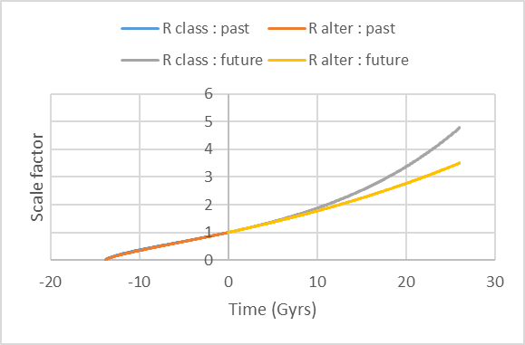
It is noteworthy that when Planck’s data (H₀ = 67.8 km/s.MPc and t_{0 =} 13.8 Gyrs) are used in Equation (10), the deduced value of « α » is :  which makes nearly a third of H₀ and is thus certainly not nil.

Figure 19 shows that the results are very close to each other using the Λ-CDM model and the present approach, at least in the past. In the future, the acceleration of the expansion would be lower with the present approach, but we shall not be there anymore to check it.

The computations also show that the acceleration starts 7.58 Gyrs after the BB in the classical model and a little bit sooner in the present approach (7.12 Gyrs) [63 ,64].

The loads/stressors in astronomical systems and in the Universe are first of all the constraints related to gravitation and energy exchanges (but could also be vacuum fluctuations, …).  

Figure 19 : Evolution of the distance scale factor R/R₀ from the Big Bang until now and in the future.

6    COMPLEX ADAPTIVE SYSTEMS AND FEEDBACK LOOPS

What is common in all these systems showing similar behaviors although they come from different disciplines : creep of metals, mechanical devices, biology, (neo-) Darwinian evolution, astronomy, cosmology ? Answer : they are complex systems adapting to constraints to which they are subjected with time going. The adaptations are the result of many positive and negative feedback loops of several orders which must occur in due time (this may be very short) for the system to maintain its integrity as a complex system. This is possible thanks to the free energy and material available in its environment.

We shall call such systems « complex adaptive systems » (CAS). A definition is given hereafter.

A preliminary remark is that this is not the usual view of complex adaptive systems as referred to in social science etc.  where partly independent (human) operators work together or in a network and give rise to an emergent complex behavior [65]. The definition proposed here has the aim to allow for quantitative description of the global (like learning, aging, evolution …) behavior of physical and biological systems as they are encountered in nature. Such systems are also adaptive and complex. However their adaptations are commonly not voluntary but structural, while their complexity results from the high number of interrelated components (as currently considered in systems theory) not as an emergent consequence of relatively simple behaviors of many people (as in complexity theory). Although these two theories have not been duly formalized yet, the publications corresponding to them show different approaches [65]. This does not preclude that the present approach might be useful for groups of human operators too.

One may define a system as a ”group of elements operating together with a common goal” [66]. Here, we define a complex adaptive system (« CAS ») as : ”a group of sub-elements operating together with a common goal and interlinked in such a way that the group shows self-organized criticality”.

Another equivalent definition is : ”A complex adaptive system is a collection of numerous interlocked subparts that is in a state of self-organized criticality such that it operates as a whole at an higher scale than that (those) of its subparts ”.

A CAS has to be seen from what we could call ”the point of view of the neutrino”. What the neutrino sees during its endless trip around the Universe are atoms which are sometimes locally more concentrated in a zone sometimes not. However, if it is a good watcher, it will not only see that atoms concentrate in zones but also that some individual atoms seem to be interlinked to each other and not (or to a much looser way, or at much lower frequencies) to other atoms present in their neighborhood.

What are the interlinks ? In most situations considered here, they can be reduced to links between atoms and molecules. This means that the sub-elements interact through the usual chemical bonds : ionic, covalent, metallic, weak bonds (Van der Waals, hydrogen, ...). Interactions may also involve information exchanges, e.g. by transmission of chemical or electric signals, ... The pattern of interlinks makes the organization of the CAS.

Complex adaptive systems can then themselves be interlinked to form bigger complex adaptive systems and so on. The links would then consist in a subtle combination of physics, chemistry and information.

The concept of self-organized criticality (or « SOC ») has been introduced by Bak and co-workers [67,68] on base of observations on sandpiles and computer simulations of cellular automata. According to this concept, many composite systems naturally evolve towards a ”critical” state characterized by four facts :

1)     minor events can be at the origin of chain reactions which can affect any number of elements in the system : therefore, ”avalanches” of events of any size can be produced;

2)     the sizes of the avalanches are distributed following a power law with a negative exponent of the order of ...1...2..;

3)     this is true as well in space as in time;

4)     when the system is constrained to produce events, it tends, thanks to the avalanches, to return to a steady state of criticality (therefore, the expression ”self-organized criticality”).

Complex adaptive systems are usually subject to constraints : due to their external environment and/or internal structure, they are not allowed to do everything. They are restricted to evolve in a limited volume, they are subjected to external and/or internal forces or stressors, they have to operate under given conditions of temperature, pressure, humidity, etc. When subject to operating conditions, the subparts and their interlinks steadily reorganize in an adaptative process saving the integrity of the complex adaptive system. Even the Universe can be seen as constrained by internal forces (gravitation) while it expands. This corresponds to the fourth item of SOC.

The adequacy of the adaptive responses will depend on the system’s internal organization and on the raw materials and energy available to carry out solutions in due time.

When one speaks of complex adaptive systems, one expects the reorganizations and adaptive responses to be characterized by several positive and negative feedback loops of any order and level of magnitude and appearing at any time.

The resulting evolution of the CAS can be modelled by the combination of all the feedback loops occurring within the subparts and between them, when time elapses.

Positive feedback loops occur e.g. when, starting from an initial state, non-standard responses are given to the challenges, i.e. responses which do not necessarily re-establish the steady state in all details. The non-standard responses can, for instance, be due to small local errors, because of the limited time available for adaptation. I say ”small” in the sense that the errors do not impair the further working of the system or the subpart : they are integrated in the further operation. But, non-standard responses can also be to the advantage of the CAS. The operating elements must continue to react in due time to the challenges with the consequence that new non-standard responses may be given. There is a cumulative effect (”snowball effect”). This makes that the mathematical expression for a first order positive feedback loop is an increasing
exponential [66] :

                              (11)

With «  » an initial value and «  » the reverse of the time constant for the response.

Positive feedback loops induce exponential growth. They are often found in the CAS under scope in this article.

Negative feedback loops correspond to re-adjustments when some characteristic of the CAS gets out of balance (e.g. because of a challenge, a shortage of material or food component, …). The balance is then re-established (e.g. homeostasis maintained in biological entities).

The mathematical expression for a first order negative feedback loop is given by [66]:

                   (12)

With « K » a constant and «  » the reverse of the time constant for the response.

First order negative feedback loops are often found in the CAS under scope of this article.

Successive first order negative feedback loops will give a concave (from below) curve which can be fitted by a power law (with ).

Higher order feedback loops will result in similar equations except when roots of negative numbers are encountered. This is e.g. the case for a second order negative feedback loop combining a first order negative feedback loop and a first order positive feedback loop as shown on Figure 20. Then the time constant for the response is given by  which means . The resulting response has then the shape of a wave [66] not of the curve of Equation (1) or part of it. This is because . Therefore one is not astonished that wavy behaviors are found in complex adaptive systems, e.g. for the TK lymphocyte activation in the immune system or with the tryptophane operon. Also, even if a little bit outside the strict definition of CAS used here, wavy behaviors appear in economy, e.g. in the management of stocks in trade [66]. These wavy behaviors are to be developed in another article (as the present article is first focused on aging / evolution curves).   

From the above, we understand that combining many positive and negative feedback loops of any order would globally result in Equation (1), except when there is a majority of wavy responses. This can be tested by computer simulations.

This is as for several laws in physics (thermodynamics, diffusion equation, …). At microscopic level, the behavior of individual particles, atoms or molecules looks erratic, but when myriads - say 10²³ - atoms or molecules act together it results in a simple global behavior at macroscopic level because of the great number. Attention was already drawn on this by Schrödinger in his book « What is Life ? » [69].    

One can consider that the same occurs at other scales. Cells are like « atoms » at the scale of an organ or body, but the combination of huge numbers of them being interlinked in the frame of a CAS shows simple global aging / evolution. Similarly, orders of 10¹¹ galaxies each with 10¹¹ stars existing in the Universe will result in a simple global evolution of it.

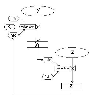
Figure 20. Schematic view of a second order negative feedback loop obtained from a first order positive feedback loop ( ( ) embedded into a first order negative feedback loop ( ).

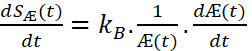
Back to biology, each individual organism is seen as a CAS. Its components and sub-components (molecules, organelles, cells, organs, sub-systems, …) are continuously subject to negative and positive feedback loops of several orders in function of the tasks they have to perform in the frame of the everyday life of the organism.

Depending on the species, a number[9] of tasks and the related feedback loops are genetically encoded : they result from natural selection and have grown into instinct. They respond to the needs of the organism and depend on the available solutions offered by the environment. The system is open as there is a continuous interaction between the organism and its environment. In default situations, the organism is genetically fully adapted to its environment. It has also several internal adaptive features allowing it to cope with external stressing agents, environmental changes, unexpected events, … Finally, thanks to their feedback loops based organization, several species have developed emerging capacities like learning, memory, …    

Considering biological entities as complex adaptive systems is consistent with (neo-)Darwinian evolution. Indeed, a first observation is that the process of natural selection itself may be seen as combining positive and negative feedback loops.

For instance, it is known that some mutations in genes may increase the adequacy of the responses to external challenges, others not. Mutations will usually appear at random in genes at a regular pace (or not) depending on the involved gene and environmental triggering factors : radiations, chemical reactions, stressing agents, ... It has in other respects been demonstrated that favourable mutations at a given locus may happen under specific stress conditions (environmental changes) much more often than in neutral conditions [70][71].

Mutations will proliferate in some genes and not or at lower pace in others (positive feedback loops). Then natural selection will favor the biological entities which are most adapted to the external challenges. Those entities whose genes allow to generate better responses (negative feedback loops) will be fitter for the challenges and thrive in their local environment.

7.  COMPLEX ADAPTIVE SYSTEMS AND ENTROPY

As Æ(t) describes the global aging / evolution behavior under constraints, it can be seen as the statistical emergence of the aging / evolution of the system. As noticed, the statistics is given by a modified Weibull distribution. Æ(t) will reflect the number of microscopic configurations of the system compatible with its macroscopic behavior at each increment of time. In line with Boltzmann’s interpretation of entropy [72], we can then define an entropy S_Æ (t) characteristic of the aging / evolving system :

                              (13)

The « entropy production », i.e. the rate of production of entropy of the system during its life will then be given by :

                       (14)

This gives using Equation (2’) :

             (15)

We see that the entropy production diminishes towards a minimum given by at time . This is in line with Prigogine’s theorem of diminution of the entropy production for dynamic open systems near to equilibrium [73]. It must be clearly emphasized that for the kind of organized CAS under scope, there is no « negentropy », nor « negative entropy » : it is the rate of increase of entropy which is decreasing not the entropy itself. The CAS takes free energy of high quality from its environment and transforms it for operation, see e.g. [74]. Then it renders the resulting degraded energy back to the environment. This allows diminution of entropy production. The 2^nd Principle of thermodynamics is thus holding all the time of the process. Entropy is increasing. But it is increasing at a still lower rate down to a minimum rate where it stays as long as possible. It is thanks to this dynamic process of diminishing the entropy production during life that information is gained [75] and organization is created.

But, after a while, there will be a risk that the entropy production starts increasing again to reach the level which would have been expected if there wouldn’t have been any dynamic CAS under scope but only an unorganized collection of the same atoms and molecules instead. The risk of increase of entropy production appears from the time . This is due to the fact that instability can occur in phenomena described by growing exponentials as soon as the exponent becomes (  in Equation (1)).

Figure 21. Illustrative example for human aging after the instability time
( : « longevity », : « lifespan », : « life expectancy »).

An example is given in Figure 21 with the aging of humans[10]. If the time  from which instability may settle (« instability time »), is 70 years, the life expectancy will lie between 70 ( ) and 140 years ( : « the longevity of the species »). With low probability of sudden death at 70 or of life until 140. Most deaths will probably be distributed between 70 and 140 in the shape of a gaussian probability curve. On Figure 21 are then mentioned: (the « lifespan ») and (the « life expectancy » for a particular sample).

The instability time gives the order of magnitude of the duration of the aging / evolution process for the CAS considered here, e.g.:

·       ~48 Gyrs for the Universe (if

·     )

·       500 – 700 Myrs for the number of taxonomic families of living beings

·       60-70 yrs for human life

·       25-30 yrs for the creep of low alloy Cr-Mo steels at 813 K

·       15-20 yrs for cars

·       10 days for flies

·       20-80 sec for the creep of carbon steels at 1473 K

·       …..

Probably, instability times for political regimes, societies, civilizations could also be inserted in such kind of table, say with values from a few dozen years to a several hundreds years ?

8.     CONCLUSION

Many observations point to a same global aging / evolution pattern of complex adaptive systems subject to constraints / stressors. The shapes of the curves are similar for a wide variety of such systems from cells to (Neo-)Darwinian evolution, from the creep of metals to the expansion of the Universe. The only difference is the order of magnitude of the duration of the phenomenon : from a few seconds for the creep of steels at 1473 K to tenths of Gyrs for the Universe. The curves can be fitted using simple general equations. The recurrent similar behavior at macroscopic level seems to be the result of self-organized patterns of interactions with huge numbers of feedback loops occurring any time at sub-macroscopic and microscopic levels. The shapes of curves referred to in the article and their translations into equations could show useful for screening several behaviors in a lot of fields in the frame of a Big History approach.  

REFERENCES :

[1] David Christian, Maps of Time: An Introduction to Big History, Berkeley, CA: University of California Press, 2nd ed., 2011

[2] Fred Spier, Big History and the Future of Humanity, 2nd ed., Malden, MA: Wiley/Blackwell, 2015

[3] Cynthia Stokes Brown, Big History: From the Big Bang to the Present, 2nd ed., New York: New Press, 2012

[4] Andrea Wulf, The Invention of Nature: The Adventures of Alexander von Humboldt, the Lost Hero of Science, (London: John Murray, 2015)

[5] H.G. Wells, Outline of History: Being a Plain History of Life and Mankind, 3rd ed., (New York: Macmillan,1921)

[6] G. U. Crevecoeur, Quantitative General Adaptation. JePublie, Paris, 2008 https://www.numilog.com/47344/Quantitative-general-adaptation.ebook

[7] G.U. Crevecoeur. An Integrated Method for Remanent Life Assessment under Creep. In Design and Analysis Methods for Plant Life Assessment, volume 112 of PVP, pages 45–56, New York, (Ed. American Society of Mechanical Engineers ASME. Pressure Vessel and Piping Conference, 1986)

[8] G.U. Crevecoeur. Über den Einsatz zerstörungsfreier und zerstörender Prüfverfahren zur Abschätzung der Restlebensdauer von Bauteilen unter dem Einfluss von Kriechen. Der Maschinenschaden, 60 (Heft1):31–40, 1987.

[9] G.U. Crevecoeur. Translation into Japanese of : Über den Einsatz zerstörungsfreier und zerstörender Prüfverfahren zur Abschätzung der Restlebensdauer von Bauteilen unter dem Einfluss von Kriechen. Kikai no songai, 33(93):15–24, 1991

 [10] G.U. Crevecoeur. Four parameters databank for full creep curve characterization. In Life Extension and Assessment: Nuclear and Fossil Power-Plant Components, volume 138 of PVP, pages 203–210, New York, (Ed. American Society of Mechanical Engineers ASME. Pressure Vessel and Piping Conference and also reference NDE 4, 1988)

[11] E.N. da C. Andrade. On the viscous flow in metals and allied phenomena. Proc. R. Soc. A, 84:1–12, 1910 [DOI 10.1098/rspa.1910.0050]

[12] G. Smith. Properties of metals at elevated temperatures. Mc Graw Hill Book Co, Inc., New York, 3 edition, 1950

[13] F.H. Norton. The Creep of Steel at High Temperatures. Ed. Mc Graw-Hill, 1929

[14] Creep data sheet. N3B. National Research Institute for Metals (NRIM), Tokyo, 1986

[15] J.T. Duane. Learning curve approach to reliability monitoring. IEEE Trans. Aerospace, 2(2):563–566, 1964 [DOI 10.1109/TA.1964.4319640]

[16] W.M. Bassin. Increasing hazard functions and overhaul policy. In Proc.1969 Ann. Symp. Reliability, 173–178, 1969

[17] R. Bell and R. Miodusky. Extension of life of US army trucks. In Proc.1976 Ann. Reliability & Maintainability Symp., pages 200–205, 1976

[18] G.U. Crevecoeur. A Model for the Integrity Assessment of Ageing Repairable Systems. IEEE Trans. Reliability, 42(1):148–155, 1993 [DOI 10.1109/24.210287]

[19] G.U. Crevecoeur. Reliability assessment of ageing operating systems. Eur. J. Mech. Eng., 39(4):219–228, 1994

[20] Junfeng Liu, Yi Wang. On Crevecoeur’s bathtub-shaped failure rate model. Computational Statistics and Data Analysis 57:645–660, 2013 [DOI 10.1016/j.csda.2012.08.002]

[21] L. Lee. Testing adequacy of the Weibull and Log linear rate models for a Poisson process. Technometrics 22 (2) : 195–199, 1980

[22] C.D. Lai, M. Xie, D.N.P. Murthy. A modified Weibull distribution. IEEE Trans. Reliab. 52 (1) : 33–37, 2003 [DOI 10.1109/TR.2002.805788]

[23] C.D. Lai, T. Moore, M. Xie. The beta integrated model. In : Proc. Int. Workshop on Reliability Modeling and Analysis—From Theory to Practice, pp. 153–159, 1998

[24] H. Selye. A syndrome produced by diverse nocuous agents. Nature, 138:32, 1936

[25] H. Selye. Studies on adaptation. Endocrinology,21(2):169–188, 1937

[26] H. Selye. Stress and the General Adaptation Syndrome. British Med. J., 1383-1392, 1950

[27] H. Selye. Stress and aging. J. Am. Geriatr. Soc., 18:669–680, 1970 [DOI 10.1111/j.1532-5415.1970.tb02813.x]

[28] H. Selye. Stress Without Distress. Ed. J.B. Lippincott Co., New York, 1974

[29] Counselling Connection (the Official Blog of the Australian Institute of Professional Counsellors). http://www.counsellingconnection.com/index.php/2009/12/10/the-general-adaptation-syndrome/

[30] Z. Shao, W. Gao, Y. Yao, Y. Zhuo, and J.E. Riggs. The dynamics of aging and mortality in the People’s Republic of China, 1957-1990. Mech. Ageing and Dev. 67:239–246, 1993 [DOI 10.1016/0047-6374(93)90002-9]

[31] A. Comfort. Ageing : The Biology of Senescence. Ed. Elsevier, New York, 1979

[32] T. Fotsis, Y. Zhang, M.S. Pepper, H. Adlercreutz, R. Montesano, P.P. Nawroth, and L. Schweigerer. The endogenous, oestrogen metabolite 2-methoxyoestradiol inhibits angiogenesis and suppresses tumour growth. Nature, 368:237–239, 1994 [DOI 10.1038/368237a0]

[33] J.E. Compston. Osteoporosis, corticosteroids and inflammatory bowel disease. Aliment. Pharmacol. Ther., 9:237–250, 1995 [DOI 10.1111/j.1365-2036.1995.tb00378.x]

[34] F. Verzar and H. Thoenen. Die Wirkung von Elektrolyten auf die thermische Kontraktion von Collagenfaden. Gerontologia, 4:112–119, 1960

[35] R.C. Young, D.L. Borden, and R.E. Rachal. Aging of the lung : pulmonary disease in the elderly. Age, 10:138–145, 1987 [DOI 10.1007/BF02432161]

[36] R.R. Willoughby. Incidental learning. J. Educ. Psychol., 20:671–682, 1929

[37] T. Matsumura, Z. Zerrudo and L. Hayflick. Senescent human diploid cells in culture : survival, DNA synthesis and morphology. J. Gerontol., 34:328–334, 1979 [DOI 10.1093/geronj/34.3.328]

[38] E.E. Baulieu. Studies of conjugated 17-ketosteroids in a case of adrenal tumor. J. Clin. Endocrinol. Metab., 22:501, 1962 [DOI 10.1210/jcem-22-5-501]

[39] N. Orentreich, J.L. Brind, R.L. Rizer and J.H. Vogelman. Age changes and sex differences in serum dehydroepiandrosterone sulfate concentrations throughout adulthood. J. Clin. Endocrinol. Metab., 59(3):551–554, 1984 [DOI 10.1210/jcem-59-3-551]

[40] M.R. Smith, B.T. Rudd, A. Shirley, P.H.W. Rayner, J.W. Williams, N.M. Duignan and P.V. Bertrand. A radioimmunoassay for the estimation of serum dehydroepiandrosterone sulphate in normal and pathological sera. Clin. Chim. Acta, 65:5–13, 1975

[41] Y. Hori, E.H. Perkins and M.K. Halsall. Decline in phytohemagglutinin responsiveness of spleen cells from aged mice. Proc. Soc. Exp. Biol. Med., 144:48, 1973 [DOI 10.3181/00379727-144-37524]

[42] M. Nei. Molecular Population Genetics and Evolution, volume 40 of Research Monographs, Frontiers of Biology. Ed. North-Holland Publishing Company, Amsterdam, 1975

[43] C. de Duve. Vital Dust. Life as a Cosmic Imperative. Ed. Basic Books, a division of HarperCollins Publishers Inc, 1995

[44] Wikipedia article, ref. : https://en.wikipedia.org/wiki/Timeline_of_the_evolutionary_history_of_life#Phanerozoic_Eon

[45] N.Eldredge and S.J. Gould. Punctuated equilibria : an alternative to phyletic gradualism. In T.J.M. Schopf, ed., Models in Paleobiology. San Francisco: Freeman Cooper, pp. 82-115, 1972. Reprinted in N. Eldredge. Time frames. Princeton: Princeton Univ. Press, pp. 193-223, 1985

[46] D.E. Kellogg. The role of phyletic change in the evolution of Pseudocubus vema (Radiolaria). Paleobiology, 1:359–370, 1975 [DOI10.1017/S0094837300002669]

[47] R.E. Lenski and M. Travisano. Dynamics of adaptation and diversification : a 10,000-generation experiment with bacterial populations. Proc. Natl. Acad. Sci. USA, 91:6808–6814, 1994 [DOI 10.1073/pnas.91.15.6808]

[48] S.F. Elena, V.S. Cooper and R.E. Lenski Punctuated Evolution caused by Selection of Rare Beneficial Mutations. Science, 272:1802–1804, 1996 [DOI 10.1126/science.272.5269.1802]

[49] Richard Lenski, E. coli Long-term Experimental Evolution Project Site, http://myxo.css.msu.edu/ecoli/index.html, last accessed February 26, 2018.

[50] Richard Lenski, Publications List, http://myxo.css.msu.edu/ecoli/publist.html#pub_2, last accessed February 26, 2018.

[51] G.U. Crevecoeur. A mechanical system interpretation of the nonlinear kinetics observed in biological ageing. Bull. Soc. Roy. Sci. Liège, 69(6):311–338, 2000

[52] G.U. Crevecoeur. A system approach modelling of the three-stage nonlinear kinetics in biological ageing. Mech. Ageing Dev., 122(3):271–290, February 2001 [DOI 10.1016/S0047-6374(00)00233-5]

[53] Max-Planck-Institut für extraterrestrische Physik – Garching (MPE-Garching). Report 2007 – 2012. Editors and Layout: W. Collmar, B. Niebisch and J. Zanker-Smith, June 2013

[54] G. Lemaître. The Beginning of the World from the Point of View of Quantum Theory. Nature, 127:706, 1931

[55] A. Einstein. Kosmologische Betrachtungen zur Allgemeinen Relativitätstheorie. Sitz. der Königlichen Preussischen Akademie der Wissenschaften zu Berlin, VI:142, 1917

[56] G.U. Crevecoeur. A system approach to the Einstein-de Sitter model of expansion of the universe. Bull. Soc. Roy. Sci. Liège, 66(6):417–433, 1997

[57] G.U. Crevecoeur. A Simple Procedure to Assess the Time Dependence of Cosmological Parameters. Phys. Essays, 12(1):115–124, March 1999 [DOI 10.4006/1.3025354]

[58] B. Schwarzschild. Very Distant Supernovae suggest that the Cosmic Expansion is speeding up. Physics Today, pages 17–19, June 1998 [DOI 10.1063/1.882267]

[59] A.G. Riess, A.V. Filippenko, P. Challis, A. Clocchiatti, A. Diercks, P.M. Garnavich, R.L. Gilliland, C.J. Hogan, S. Jha, R.P. Kirschner, B. Leibundgut, M.M. Phillips, D. Reiss, B.P. Schmidt, R.A. Schommer, R. Chris Smith, J. Spyromilio, Ch. Stubbs, N.B. Suntzeff, and J. Tonry. Observational Evidence from Supernovae for an Accelerating Universe and a Cosmological Constant. Astron. J., 116:1009–1038, September 1998 [DOI 10.1086/300499]

[60] S. Perlmutter, G. Aldering, G. Goldhaber, R.A. Knop, P. Nugent, P.G. Castro, S. Deustua, S. Fabbro, A. Goobar, D.E. Groom, I.M. Hook, A.G. Kim, M.Y. Kim, J.C. Lee, N.J. Nunes, R. Pain, C.R. Pennypacker, R. Quimby, C. Lidman, R.S. Ellis, M. Irwin, R.G. McMahon, P. Ruiz-Lapuente, N. Walton, B. Schaefer, B.J. Boyle, A.V. Filippenko, T. Matheson, A.S. Fruchter, N. Panagia, H.J.M. Newberg, and W.J. Couch. Measurements of Omega and Lambda from 42 High-Redshift Supernovae. Astrophys. J., 517:565–586, June 1999 [DOI 10.1086/307221]

[61] C.L. Bennett, L. Larson, J.L. Weiland, N. Jarosk et al. Nine-Year Wilkinson Microwave Anisotropy Probe (WMAP) Observations: Final Maps and Results. The Astrophysical Journal Supplement 208 (2): 20,[arXiv:1212:5225], 2013 [DOI 10.1088/0067-0049/208/2/20]

[62] Planck collaboration. Planck 2015 results. I. Overview of products and scientific results. Astronomy & Astrophysics manuscript, [arXiv :1502.01582v2 astro-ph.CO], 10 Aug 2015

[63] G. U. Crevecoeur. Evolution of the distance scale factor and the Hubble parameter in the light of Planck’s results, [arXiv:1603.06834v2 physics.gen-ph], 15 Feb 2017

[64] G.U. Crevecoeur. Time evolution of dark energy and other cosmological parameters. Phys. Essays, 30(3):255–263, September 2017 [DOI 10.4006/0836-1398-30.3.255]

[65] Phelan, S.E. A Note on the Correspondence Between Complexity and Systems Theory. Systemic Practice and Action Research, Vol. 12, No. 3, 237-246, 1999 [DOI 10.1023/A:1022495500485]

[66] J.W. Forrester. Principles of Systems. Ed. Wright-Allen Press, 1968

[67] P. Bak, C. Tang, and K. Wiesenfeld. Self-organized criticality : an explanation of 1/f noise. Phys. Rev. Lett., 59:381–384, 1987 [DOI 10.1103/PhysRevLett.59.381]

[68] P. Bak, C. Tang, and K. Wiesenfeld. Self-organized criticality. Phys. Rev. A, 38(1):364–374, 1988 [DOI 10.1103/PhysRevA.38.364]

[69] E. Schrödinger. What is Life ? Cambridge University Press, 1967

[70] J. Cairns, J. Overbaugh and S. Miller. The origin of mutants. Nature, 335:142–145, 1988 [DOI 10.1038/335142a0]

[71] B.G. Hall. Spontaneous point mutations that occur more often when advantageous than when neutral. Genetics, 126:5–16, 1990

[72] L. Boltzmann. Entgegnung auf die wärmetheoretischen Betrachtungen des Hrn. E. Zermelo. Wiedermann Ann., 57:773–784, 1895

[73] I. Prigogine. Introduction to Thermodynamics of Irreversible Processes. Ed. Interscience Publishers, New York, 2 edition, 1961

[74] E. Chaisson, Cosmic Evolution: The Rise of Complexity in Nature, Cambridge, MA: Harvard University Press, 2001

[75] D. Layzer. The arrow of time. Scientific American, 12:56–69, 1975